Automatic Wildfire Smoke Detection Using Deep Learning

Hi friendly reader! My name is Aristana Scourtas, and I’m currently pursuing my MS in Artificial Intelligence at Northwestern University. I have two years of industry software experience and a dream to apply my computing skills to environmental and climate change-related issues. This summer I’m committed to finding novel solutions to an old problem — early detection of wildfires.

Fire moves fast

The early detection of smoke from wildfires is critical to saving lives, infrastructure, and the environment — and every minute counts. Once ignited, a fire can spread at speeds of up to around 14 mph1 — that’s about 2.3 miles every 10 minutes! The devastating Camp wildfire that tore through northern California in 2018 moved at more than a football field per second (160 ft/s) at its fastest point.2

The Camp Wildfire (Nov 8th, 2018), imaged via Landsat 8, a NASA/USGS satellite.3

So how can we do this? Currently, wildfires are detected any number of ways: in California, wildfires are typically first recorded via 911 (a US emergency hotline) calls4, but we also detect wildfires via fire watchtowers or by camera networks and satellite images (like from the GOES5 or VIIRS6 satellites) that inspect areas of interest. In all of these cases, a person needs to continually monitor the data streams for signs of smoke and fires.

However, human beings can only do so much. Continuously monitoring multiple video feeds for fires is a fatiguing, error-prone task that would be challenging for any person.

But how about a computer?

What deep learning can do

Deep learning is a subset of machine learning that focuses specifically on neural networks with a high number of layers. Machine learning is really good at doing things humans are typically bad at, like rapidly synthesizing Gigabytes of data and finding complicated patterns and relationships.

A simple neural network with only one hidden layer. We’d call this a “shallow” neural network. (Graphic modified from V. Valkov)8

Neural networks are said to be “universal approximators”,7 because they can learn any nonlinear function between an input and an output — this is very helpful for analyzing the patterns and relationships in images, for example.

Deep learning algorithms are good for the task of smoke detection, because they can constantly and automatically “monitor” the image and video streams from fire watchtower networks and satellites, and alert officials when there’s likely smoke in the image.

Current algorithms

As I’m writing this article, the current research out there on deep learning for wildfire smoke detection largely focuses on using Convolutional Neural Networks (CNNs) for static images. CNNs are commonly used for image data, and are good at learning spatial information.

For example, in my smoke detection research, we’re working with an image dataset from the HPWREN9 tower network in southern California.

An example HPWREN image capturing smoke. This image, after it is pre-processed for the neural network, is then fed to the CNN as input.

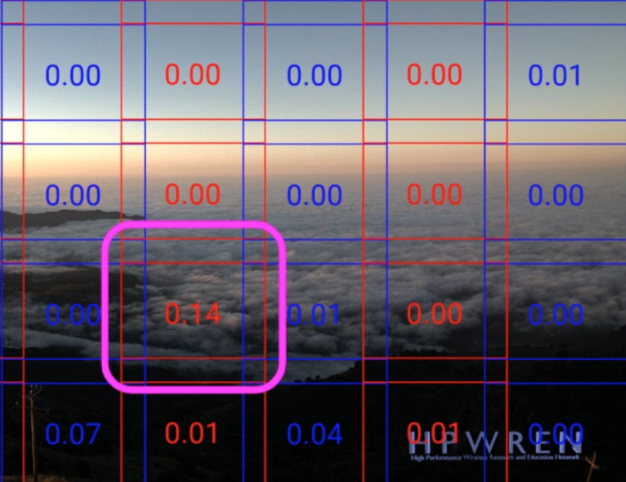
Unfortunately, while these CNN-based algorithms usually have high accuracy, they can also produce a high number of false positives, meaning they mistake other things, like clouds or fog, for smoke.

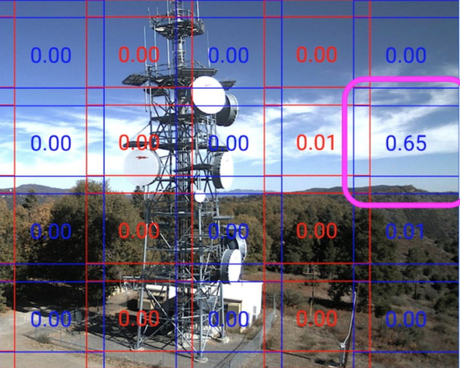
Examples of false positives from the work of Govil et al in their 2020 paper. This model divided the image into a grid, and assigned the likelihood of each grid cell being smoke (the threshold for smoke was adjusted dynamically).4 On the left, clouds were mistaken for smoke. On the right, fog was mistaken for smoke.

Furthermore, while these models do well in their studies, oftentimes they do not perform well when assessed with images from other regions. For instance, the ForestWatch model, which has been deployed in a variety of countries such as South Africa, Slovakia, and the USA, did not perform well when assessed using data from Australian watch towers.10

This begged the question: “well, how do humans detect wildfire smoke?” Looking through the dataset of images of California landscapes, I often found I could not tell if there was smoke in any of the early images.

Can you find the smoke in this image from the HPWREN towers? It was taken 9 minutes after the smoke plume was confirmed to be visible from the tower.
(Answer: from the left of the image, it’s 1/3 of the way in)

I’d only see the smoke once I compared images sequentially, from one timestamp to the next. Intuitively, movement on or below the horizon seemed to be a key aspect of recognizing smoke.

Is time the secret ingredient?

After listening to the opinions of my mentors and a California fire marshal, it seemed like everyone agreed — movement was a key part of how we identified smoke.

Could we create a model that learns temporal information as well as spatial information? In other words, could it learn both what smoke looked like (spatial), and how the images of smoke changed over time (temporal)?

I’m now developing an algorithm that can do just that. Often, a Long Short-Term Memory network (LSTM), which is a kind of Recurrent Neural Network (RNN), are used for learning patterns over time (i.e. in sequential data). For instance, LSTMs are frequently used for text prediction and generation (like that in the Messages app on iPhones).

Models that combine spatial data (often learned via CNNs) with some other model or technique that captures temporal data have been used in a variety of other applications with video or sequential image data, such as person re-identification, object tracking, etc.

We’re exploring how we can apply a similar hybrid spatial-temporal model to our smoke dataset.

Conclusion

Automated early detection of wildfire smoke using deep learning models has shown promising results, but false positive rates remain high, particularly when the models are deployed to novel environments.

Including a temporal component may be a key way we can improve these models, and help them distinguish better between smoke and clouds or fog.

This work doesn’t come a moment too soon, as wildfires are increasing in intensity and frequency due to climate change’s effects on air temperature, humidity, and vegetation, among other factors. Unfortunately, fires like the ones that tore across Australia earlier this year will become much more common in many parts of the globe.

Hopefully, as we improve the technology to detect these fires early on, we can save lives and ecosystems!

The Amazon Rainforest, home to many peoples and countless species. A home worth protecting.

References

  1. “How Wildfires Work”. https://science.howstuffworks.com/nature/natural-disasters/wildfire.htm
  2. “Why the California wildfires are spreading so quickly”. https://www.cnn.com/2018/11/09/us/wildfires-why-they-spread-so-quickly-wcx/index.html
  3. Camp Fire photo. https://en.wikipedia.org/wiki/Camp_Fire_(2018)
  4. Govil, K., Welch, M. L., Ball, J. T., & Pennypacker, C. R. (2020). Preliminary Results from a Wildfire Detection System Using Deep Learning on Remote Camera Images. Remote Sensing12(1), 166. https://www.mdpi.com/2072-4292/12/1/166
  5. GOES. https://www.nasa.gov/content/goes-overview/index.html
  6. VIIRS. https://ncc.nesdis.noaa.gov/VIIRS/
  7. Scarselli, F., & Tsoi, A. C. (1998). Universal approximation using feedforward neural networks: A survey of some existing methods, and some new results. Neural networks11(1), 15-37. https://www.sciencedirect.com/science/article/pii/S089360809700097X?casa_token=NaZxQdSUi6MAAAAA:zMhRIkTNDTZWSWze5wIHVK73EtlgHzLm3cAMkRBpQmepxH3cSAyhIvPKpu_H5b-2kYdTcG1IQA
  8. NN graphic. https://towardsdatascience.com/build-a-simple-neural-network-with-tensorflow-js-d434a30fcb8
  9. HPWREN. http://hpwren.ucsd.edu/cameras/
  10. Alkhatib, A. A. (2014). A review on forest fire detection techniques. International Journal of Distributed Sensor Networks10(3), 597368. https://journals.sagepub.com/doi/full/10.1155/2014/597368
  11. Amazon Rainforest photo. https://www.telegraph.co.uk/travel/destinations/south-america/articles/the-amazon-travel-guide/

Digitalize Argonne National Lab

Author: James Shengzhi Jia, Northwestern University, rising sophomore in Industrial Engineering & Management Science

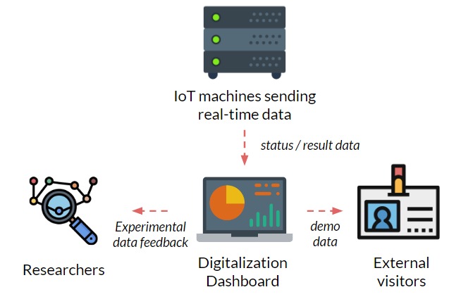
Imagine if you are a researcher here at Argonne, and you don’t have to go  upstairs downstairs all the time just to check the experiments that you are running — all you have to do is sit in front of the computer, monitor and control all of them in one system. Wouldn’t that be amazing?

Figure 1: Schematic of the project motivation

Before this internship, I couldn’t possibly imagine such a scenario. However, during the summer, I was working with my mentor Jakob Elias at Energy and Global Security Directorate and creating the beta infrastructure of the system that can connect and visualize real-time data from IoT machines at Argonne, and achieve automatic optimization of experiments.
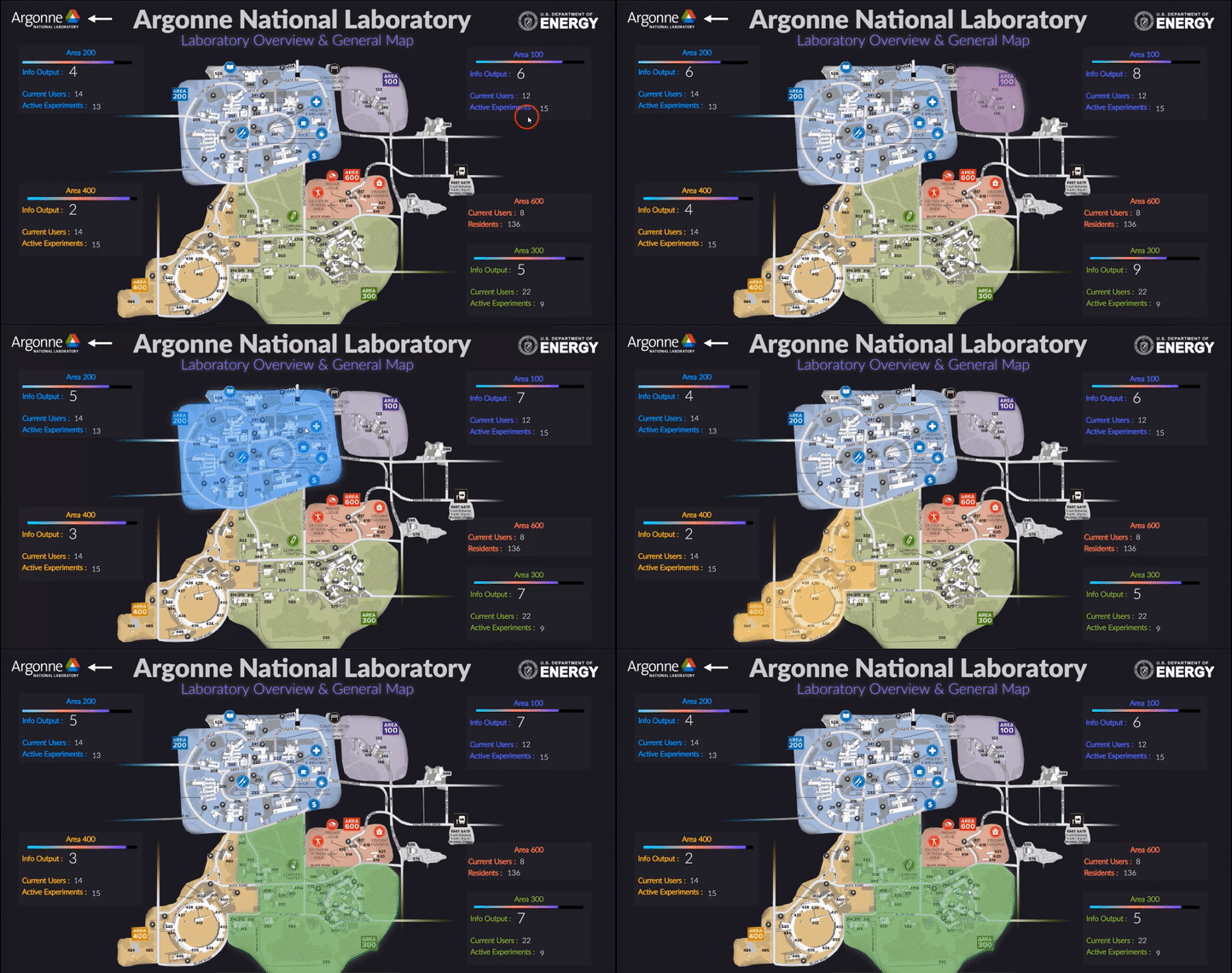
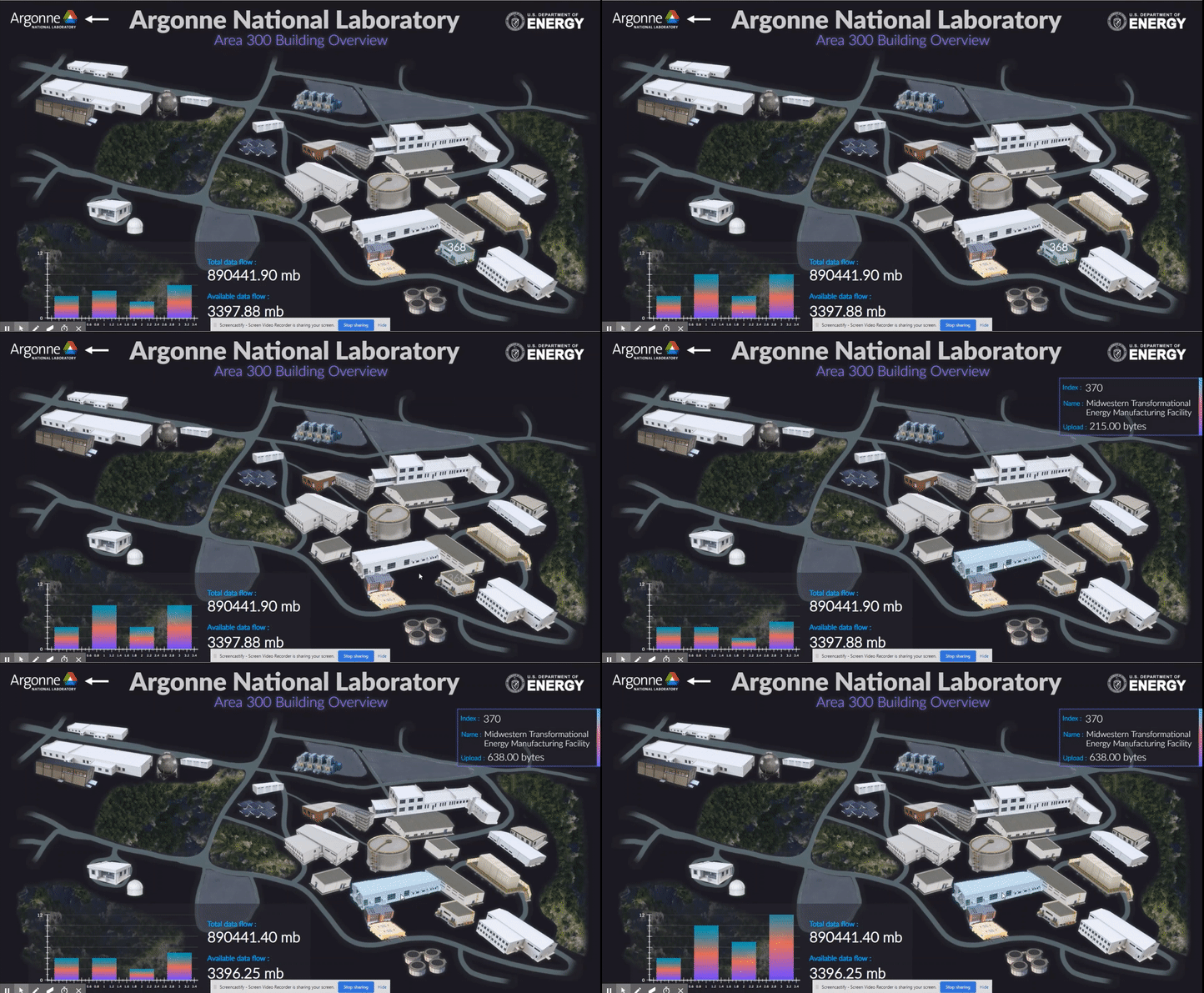
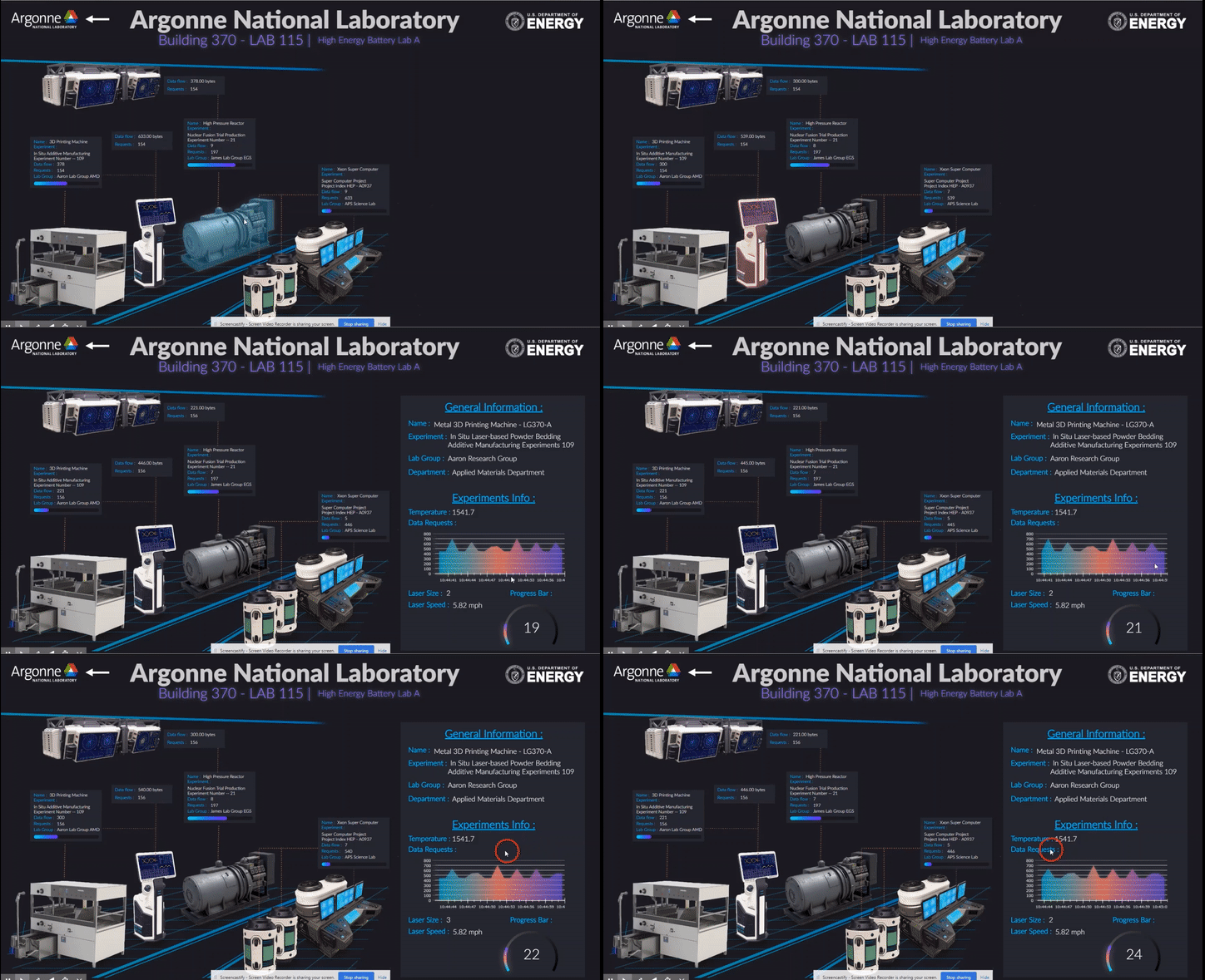
The following short videos demonstrated the beta infrastructure that I created. It’s easy to navigate through the interactive map, and obtain key information about the areas, buildings, rooms and experiments that are of your interest. The dashboard is able to receive data from the local system, websites and also MQTT protocol. In the future, we plan to integrate various AI applications into the dashboard, so it becomes even smarter and grants researchers full control of their experiments right in their office. 
The second part of my work is testing the usability of this dashboard by using the metal 3D printing experiment in Applied Materials Department (AMD) as a test case. Let me give you a brief introduction of the experiment and their objective:  (Full explanation can be seen in Erkin Oto’s past post)

AMD researchers at Argonne utilize powerful laser beam, X-ray and IR to conduct metal 3D printing experiments, and the key objective is to characterize and identify the product defects. However, as X-ray machines (which are used to identify defects) are not as ubiquitous as IR machines, researchers at Argonne are exploring whether it’s possible to only use IR data to identify the defects in the products. 

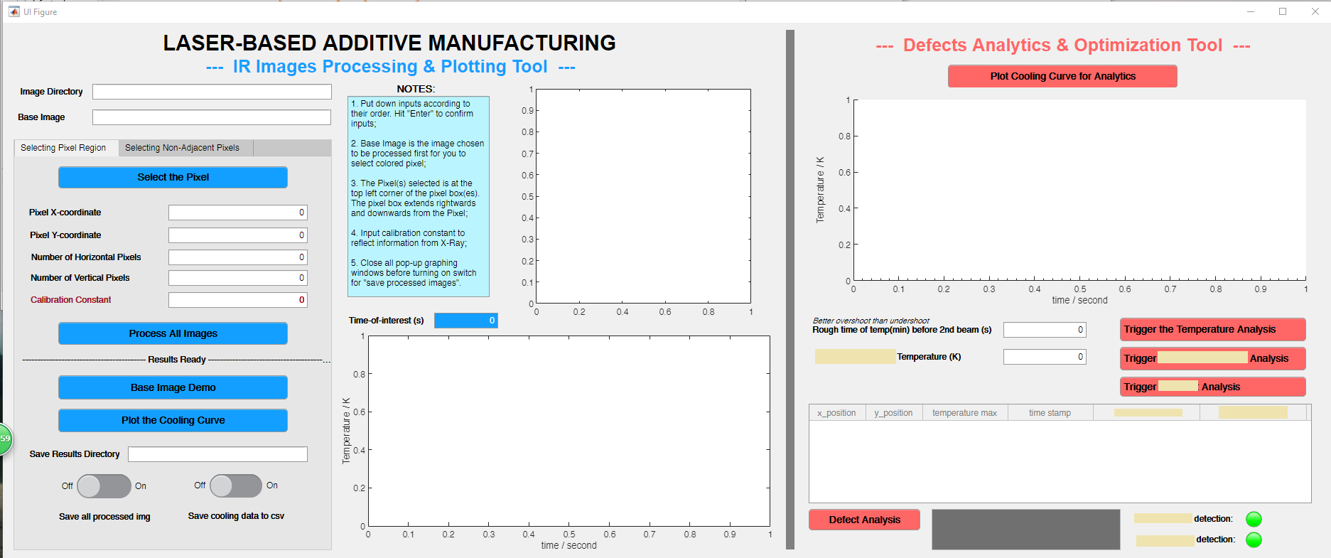
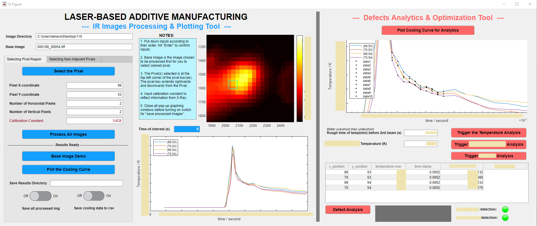
Firstly, as each experiment generates over 1000 IR images, I created a MATLAB software that speeds up the analysis of those images to just within 10 seconds. As shown below, the software works to transform an original black IR image to a fully colored image that researchers can select pixels-of-interest on.
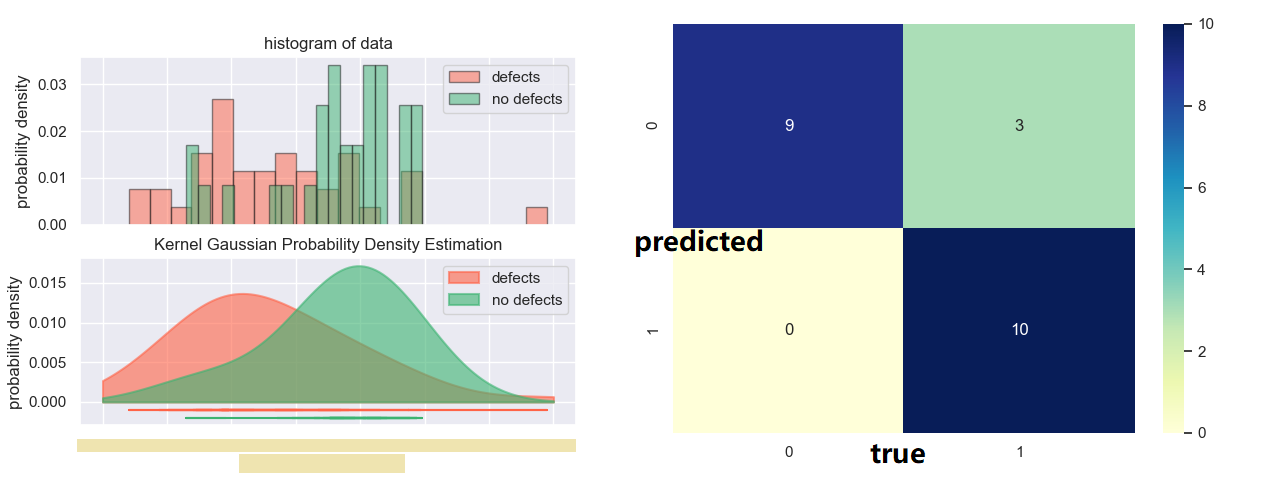
Secondly, additional to the processing tool, I also programmed an analytical tool (which can be seen below) to quantitatively analyze the defect / non-defect dataset. In the process, I came up with two original methods to investigate the correlation, and applied Kernel Gaussian PDF Estimation, Mann-Whitney U Test, and Machine Learning via logistic regressionBased on the original methods that I developed and therefore the machine learning model trained, the accuracy of the model reaches 86.3%, with p values for both method coefficient below 0.1. 
In the future, more efforts can be put into obtaining more accurate data, to improve the model. In a bigger picture, we can also explore about integrating applications like this into the dashboard, and achieve the digitalization of Argonne National Lab in the near future.
Disclaimer: all blocked image data are intended to protect the confidentiality of this project. Unblocked data are either trivial or purely arbitrary (such as ones in prototype dashboard).

Optimizing Neural Network Performance for Image Segmentation

Hi! My name is Joshua Pritz. I’m a rising senior studying physics and math at Northwestern University. This summer, I am working with Dr. Marta Garcia Martinez in the Computational Science Division at Argonne National Lab. Our research concerns the application of Neural Network based approaches to the semantic segmentation of images detailing the feline spinal cord. This, too, is part of a larger effort to accurately map and reconstruct the feline spinal cord with respect to its relevant features – namely, neurons and blood vessels.
Prior to outlining my contribution to this work, it’s worth introducing the terminology used above and, thereafter, illustrating why it fits the motivations of our project. Image segmentation, generally, is the process of identifying an image’s relevant features by distinguishing its regions into different classes. In the case of our cat spine dataset, we are currently concerned with two classes: somas, the bodies of neurons in the spine, and background, everything else. Segmentation can be done by hand. Yet, with over 1800 images collected via x-ray tomography at Argonne’s Advanced Photon Source, this task is all but intractable. Given the homogeneity of features within our images, best exemplified by the similarity of blood vessels and somas (indicated in Figure 1 by a blue and red arrow, respectively), traditional computer segmentation techniques like thresholding and K-means clustering, which excel at identifying objects by contrast, would also falter in differentiating these features.
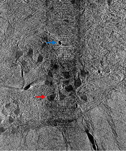
Figure 1: Contrast adjusted image of spinal cord. Blue arrow indicates blood vessel, while red arrow indicates soma.
Enter the Convolutional Neural Network (CNN), through which we perform what is known as semantic segmentation. Herein, a class label is associated with every pixel of an image. A CNN begins by assigning a trainable parameter, a weight, to each pixel in an incoming image. Then, in a step known as a convolution, it performs an affine operation on each submatrix of pixels in the image using a fixed scaling matrix called the kernel, which is then translated using another set of trainable parameters called biases. Convolutions create a rich feature map that can help to identify edges, areas of high contrast, and other features depending on the kernel used. Such operations also reduce the number of trainable parameters in succeeding steps, which is particularly helpful for large input images that necessarily subtend hundreds of thousands of weights and biases. Through activation functions that follow each convolution, the network then decides whether or not objects in the resultant feature map correspond to distinct classes.
This seems like a complicated way to perform an intuitive process, surely, but it begs a number of simple questions. How does the network know whether or not an object is in the class of interest? How can it know what to look for? Neural networks in all applications need to be trained extensively before they can perform to any degree of satisfaction. In the training process, a raw image is passed through the CNN. Its result – a matrix of ones and zeros corresponding respectively to our two classes of interest – is then compared to the image’s ground truth, a segmentation done by hand that depicts the desired output. In this comparison, the network computes a loss function and adjusts its weights and biases to minimize loss throughout training, similar to the procedure of least-squares regression. It takes time, of course, to create these ground truths necessary for training the CNN, but given the relatively small number of images needed for this repeatable process, the manual labor required pales in comparison to that of segmentation entirely by hand.
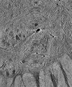
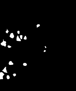
Figure 2: Cat spine image and its ground truth.

The question then becomes, and that which is of primary concern in this research, how can training, and the resulting performance of the CNN, be optimized given a fixed amount of training data? This question lives in a particularly broad parameter-space. First, there are a large number of tunable network criteria, known as hyperparameters (so as not to be confused with the parameters that underlie the action of the CNN), that govern the NN’s performance. Notably, these include epochs, one full pass of the training data through the network; batch-size, the number of images seen before parameters are updated; and learning rate, the relative amount parameters are updated after each training operation. For our network to perform exceptionally, we need to include enough epochs to reach convergence (the best possible training outcome) and tune the learning rate so as to meet it within a reasonable amount of time, while not allowing our network to diverge to a poor result (Bishop).
Second, we can vary the size of images in our training set, as well as the number of them. Smaller images, which are randomly cropped from our full-sized dataset, require a fewer number of trainable weights and biases, thus exhibiting quicker convergence. Yet, such images can neglect the global characteristics of certain classes, resulting in poorer performance on full-sized images. In choosing a number of images for our training set, we need balance whether or not enough data is present to affect meaningful training with oversampling of training data. To conclusively answer our project’s primary question without attempting to address the full breadth of the aforementioned parameter space, we developed the following systematic approach.
Prior to our efforts in optimization, we added notable functionality to our initial NN training script, which was written by Bo Lei of Carnegie Mellon University for  the segmentation of materials science images and, herein, adapted to perform on our cat spine dataset. It employs the PyTorch module for open-source accessibility and uses the SegNet CNN architecture, which is noteworthy for its rendering of dense and accurate semantic segmentation outputs (Badrinarayanan, Kendall and Cippola). The first aspect of our adaptation of this script that required attention was its performance on imbalanced datasets. This refers to the dominance of one class, namely background, over a primary class of interest, the somas. To illustrate, an image constituted by 95 percent background and five percent soma could be segmented with 95 percent accuracy, a relatively high metric, by a network that doesn’t identify any somas. The result is a network that performs deceptively well, but yields useless segmentations. To combat this, our additional functionality determines the proportion made up by each class across an entire dataset, and scales the loss criterion corresponding to that class by the inverse of this proportion. Hence, loss corresponding to somas is weighted more highly, creating networks that prioritize their identification.
We also include data augmentation capabilities. At the end of each training epoch, our augmentation function randomly applies a horizontal or vertical flip to each image, as well as random rotations, with fifty percent probability. These transformed images, although derived from the same dataset, activate new weights and biases, thereby increasing the robustness of our training data. Lastly, we added visualization functionality to our script, which plots a number of metrics computed during training with respect to epoch. These metrics most notably include accuracy, the number of pixels segmented correctly divided by the total number of pixels, and the intersection-over-union score for the soma class, the number of correctly segmented soma pixels divided by the sum of those correctly identified with the class’s false positive and negatives (Jordan). We discuss the respective significance of these metrics insofar as evaluating a segmentation below.
Table 1: Hyperparameters used in training.

After including such functionalities our interest turned to optimizing the network’s hyperparameters as well as the computational time needed for training. To address the former, we first trained networks using our most memory-intensive dataset to determine an upper bound on the number of epochs needed to reach convergence in all cases. For the latter, we conducted equivalent training runs on the Cooley and Bebop supercomputing platforms. We found that Bebop offered an approximately two-fold decrease in training time per epoch, and conducted all further training runs on this platform. The remainder of the hyperparameters, with the exception of learning rate, are adapted from Stan et al. who perform semantic segmentation on similar datasets in MATLAB. Our preferred learning rate in this case was determined graphically, whereby we found that a rate of 10-4 did not permit effective learning during training on large images, while a rate of 10-2 led to large, chaotic jumps in our training metrics.
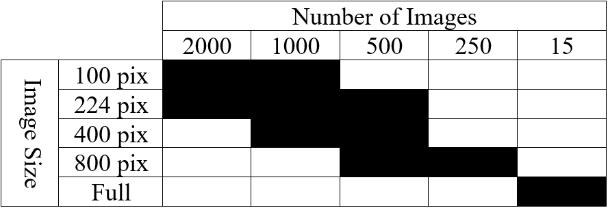
Table 2: List of tested cases depicting image size and number of images in training set.
Using such hyperparameters, listed in Table 1, for all successive training, we finally turned our attention to optimizing our networks’ performance with respect to the size of training images as well as the number of them used. Our initial training images (2300 by 1920 pixels) are very large compared to the size of images typically employed in NN training, which are in the ballpark of 224 by 224 pixels. Likewise, Stan et al. find that, despite training NNs to segment larger images, performance is optimal when using 1000 images of size 224 by 224 pixels. To see if this finding holds for our dataset, we developed ten cases that employ square images (with the exception of full-sized images) whose size and number are highlighted in Table 2. Image size varies from 100 pixels to 800 pixels per side, including training conducted on full-sized images, while image number varies from 250 to 2000. In this phase, one NN was trained and evaluated for each case.
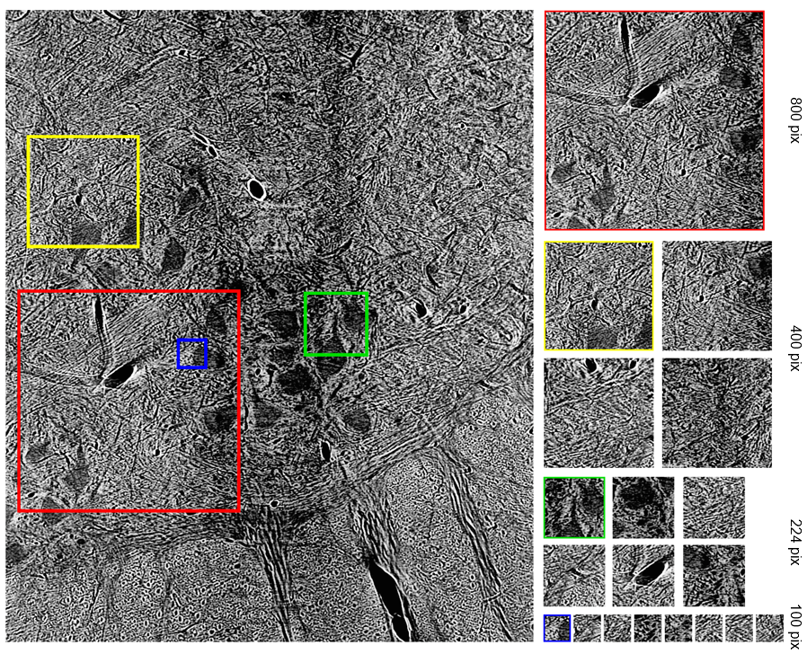
Figure 3: Detail of how smaller images were randomly cropped from full-sized image.
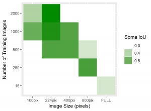
To standardize the evaluation of these networks, we applied each trained NN to two x-ray tomography test images. Compared to the 20+ minutes needed to segment one such image by hand, segmentation of one such 2300 by 1920 pixel image took averagely 12.03 seconds. Resulting from each network, we recorded the global accuracy, soma intersection-over-union (IoU) score, and boundary F-1 score corresponding to each segmentation. Accuracy is often high for datasets whose images are dominated by background, such is the case here, and rarely indicates the strength of performance on a class of interest. Soma IoU, on the other hand, is not sensitive to the imbalance in classes exhibited by our dataset. The boundary F-1 (BF1) score for each image is related to how close the boundary of somas in our NN segmentation is to that of the ground truth. Herein, we use a threshold of 2 pixels, so that if the boundary in our NN’s prediction remains within 2 pixels of the actual soma boundary, the segmentation would receive a 100% BF1 score (Fernandez-Moral, Martins and Wolf). Together with the soma IoU, these metrics provide a far more representative measurement of the efficacy of our network than solely global accuracy. For each network, we exhibit the average of these metrics over both test images in the table below, in addition to heatmaps for soma IoU and BF1 scores.
Figure 4: Heatmaps for BF1 and Soma IoU score for each case.
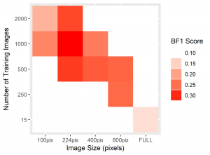

Table 3: Results from test image segmentations.
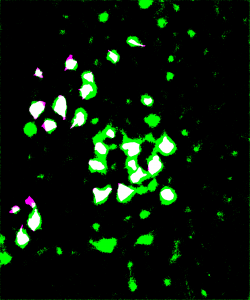
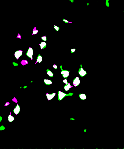
To visually inspect the quality of our NNs’ output, we overlay the predictions given by each network with the ground truth for the corresponding test image using a MATLAB script developed by Stan et al. This process indicates correctly identified soma pixels (true positives) in white and correctly identified background pixels in black (true negatives). Pink pixels, however, indicate those falsely identified as background (false negatives), while green pixels are misclassified as somas (false positives). We exhibit overlays resulting from a poorly performing network as well as those from our best performing network below.
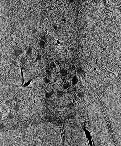
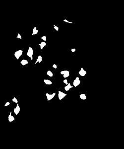
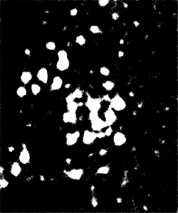
Figure 5: Top: raw test image (left) and test image ground truth (right). Bottom: NN (poorly performing) prediction (left) and overlay of prediction with ground truth (right).
The heatmaps above detailing soma IoU and BF1 scores visually represent trends in network performance with respect to image size and number. We recognize the following. The boundary F-1 score generally decreases when increasing the number of images in the training set. This is most likely due to oversampling in training data, by which resultant networks become too adept in performing on their training data and lose transferability that allows them to adapt to the novel test images. We recognize a similar trend in soma IoU. More so, network performance is seen to appreciate as we decrease the size of training images, until it reaches a maximum in the regime of 224 by 224 pixel images. The decrease in performance of networks trained on larger images may be explained by the lack of unique data. Despite a comparable number of training images, datasets of a larger image size are likely to have sampled the same portion of the original training images multiple times, resulting in redundant and ineffective training. The 100 by 100 pixel training images, on the other hand, are likely too small to capture the global character of somas in a single image given that some such features often approach 100 by 100 pixels in size. Hence, larger images may be needed to capture these essential morphological features. We find that highest performing network is that which was trained using 1000 images of size 224 by 224 pixels, exhibiting a global accuracy of 98.1%, a soma IoU of 68.6%, and a BF1 score of 31.0%. The overlay corresponding to this network shown in Figure 6 depicts few green and pink pixels, indicating an accurate segmentation.


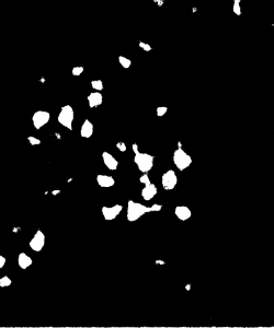
Figure 6: Top: raw test image (left) and test image ground truth (right). Bottom: NN (224pix1000num – best performing) prediction (left) and overlay of prediction with ground truth (right)
Ultimately, this work has shown that convolutional neural networks can be trained to distinguish classes from large and complex images. NN based approaches, too, provide an accurate and far quicker alternative to manual image segmentation and past computer vision techniques, given an appropriately trained network. Our optimization with respect to the size and number of images used for training has confirmed the findings of Stan et al. in showing that networks trained using a larger amount of smaller images perform better than those trained using full-sized images. Namely, our results indicate that 224 by 224 pixel images yield the highest performance with respect to accuracy, IoU, and BF1 scores. In the future, this work may culminate in the application of our best NN to the totality of the feline spinal cord dataset. With appropriate cleaning and parsing of the resultant segmentations, such a network could aid in novel 3D reconstructions of neuronal paths in the feline spinal cord.

References

Badrinarayanan, Vijay, Alex Kendall and Roberto Cipolla. “SegNet: A Deep Convolutional Encoder-Decoder Architecture for Image Segmentation.” IEEE Transactions on Patter Analysis and Machine Intelligence (2017): 2481-2495. Print.
Bishop, Christopher M. Pattern Recognition and Machine Learning. Cambridge: Springer, 2006. Print.
Fernandez-Moral, Eduardo, et al. “A New Metric for Evaluating Semantic Segmentation: Leveraging Global and Contour Accuracy.” 2018 IEEE Intelligent Vehicles Symposium (IV) (2018): 1051-1056. Print.
Jordan, Jeremy. “Evaluating Image Segmentation Models.” Jeremy Jordan, 18 Dec. 2018, www.jeremyjordan.me/evaluating-image-segmentation-models/. Website.
Stan, Tiberiu, et al. Optimizing Convolutional Neural Networks to Perform Semantic Segmentation on Large Materials Imaging Datasets: X-Ray Tomography and Serial Sectioning. Northwestern University, 19 June 2019. Print.

Using Time Series Techniques to Understand the Correlation between Light, Thermal Radiation, and Reported Temperature Error

Hello! My name is Kevin Mendoza Tudares, and I am a rising sophomore at Northwestern University studying Computer Science. This summer, I am working with Pete Beckman and Rajesh Sankaran on developing a process to clean and organize preexisting and incoming data from the Array of Things (AoT) nodes as well as use time series techniques on this data to quantify the correlation between direct exposure to sunlight and the resulting error in the reported environmental temperature (and humidity) by the node.
Having an up-to-date server and database is critical when working with live and time-series data, and at the moment, the research team is transitioning their database system to using PostgreSQL extended with TimescaleDB in order to efficiently manage the incoming data from the nodes as time-series data. That is why a part of what I am working on this summer is writing scripts/programs that will cleanly create mappings and upload data representing the system of nodes and sensors in the form of .csv files into their appropriate relational tables in the new database. These scripts will also transfer other preexisting node and sensor data along with large amounts of measurement data from the previous database system into the new one. This first part of my work is important for the execution of the second portion as I will be working with this same data to find correlations between the reported solar exposure and error in reported temperature.
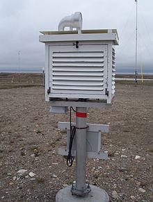
The second task I will be working on involves knowledge of thermal radiation and how it affects the performance of outdoor temperature instruments, such as those used in climatology stations and found usually in white plastic housings or enclosures called Stevenson screens. These enclosures protect the instruments from precipitation and direct or reflected sunlight while still allowing air to circulate through them, thus allowing more accurate and undisturbed measurements from the environment around them. AoT nodes are built in a similar fashion for the same benefits, as seen in the figures below.

Figure 1: An AoT Node  

      Figure 2:  Exterior of a Stevenson screen

Along with the benefits of protection from this design, one of the issues with this for the AoT node enclosure is the concept of solar gain, which is the increase in thermal energy, or heat, in a space or object as it absorbs solar radiation. While the node casing protects the temperature sensors from direct incident radiation, as none of it is transmitted directly through the material and most of the radiation is reflected, there is still the presence of thermal reradiation from the protective material. This is because “despite being coloured white the external surfaces may be free to absorb some short-wave radiation, and some of this may reradiate internally” into the node as long-wave radiation and onto the temperature sensors (Burton 160). This infrared radiation causing the error doesn’t need to come from the sun directly, as it could also come from the glare from glass of a nearby building or from the hood of a passing vehicle, but this error is most often to occur in the day time when the sun is out and shining directly on these nodes. Another issue that goes in hand with the thermal reradiation would be the size of these nodes, as previous research has found that an overheating of air temperature inside smaller sized Stevenson screens was detected more frequently in comparison to much larger Stevenson screens, and these findings could be applied to the small-scale nodes mounted on poles (Buisan et al. 4415). Excessive solar gain can lead to overheating within a space, and with less space, this form of passive heating is much more effective as the heat cannot disperse. Finally, one last issue with the internal temperature of the nodes is the lack of active ventilation. Studies have found that Stevenson screens that are non-aspirated (no ducts) reported significantly warmer internal temperatures than ones with aspiration ducts under low wind conditions (Hoover and Yao 2699). Without aspiration ducts, which all nodes lack, the cooling for these nodes to maintain them at ambient temperature is limited to only wind conditions that will circulate air through the node.
Thus, with the knowledge of potential issues with the nodes that could result in errors in ambient temperature data, my task is to find, understand, and quantify the described trend. This process will involve the time-series data I previously cleaned and uploaded, querying the detected visible and infrared light measurement data from a node at times where the calculated temperature error reaches a certain magnitude, and using these associated values to create a model. This model can then be applied to estimate a more accurate measurement of the ambient temperature around the node by accounting for this error at other times given the light measurements.
My work on this project is important because working with accurate data and readings is essential for all other data analysis and machine learning tasks that must be done by the team to identify and predict phenomena in our environment. For this to be done, we must have faith in the data and any trends we see, and I am contributing to help understand these trends and account for them. Special thanks to Pete Beckman, Rajesh Sankaran, and Jennifer Dunn for mentoring me this summer.
 
References:
Buisan, Samuel T., et al. “Impact of Two Different Sized Stevenson Screens on Air Temperature Measurements.” International Journal of Climatology, vol. 35, no. 14, 2015, pp. 4408–4416., doi:10.1002/joc.4287.
Burton, Bernard. “Stevenson Screen Temperatures – an Investigation.” Weather, vol. 69, no. 6, 27 June 2014, pp. 156–160., doi:10.1002/wea.2166.
Hoover, J., and L. Yao. “Aspirated and Non-Aspirated Automatic Weather Station Stevenson Screen Intercomparison.” International Journal of Climatology, vol. 38, no. 6, 9 Mar. 2018, pp. 2686–2700., doi:10.1002/joc.5453.